Statistical Distributions Unleashed with Python Code.

In a world of statistics a data distribution is a function which presents all the possible values of the data. It also shows how often each value occurs.
From this distribution it is possible to calculate the probability of any one particular observation in the sample space, or the likelihood that an observation will have a value which is less than (or greater than) a point of interest.
The function of a distribution that presents the density of the values of our data is called a probability density function or simply pdf.

Gaussian (normal) distribution:

The Gaussian distribution, also known as the normal distribution or bell curve, is a fundamental concept in the world of statistics and probability. It is a continuous probability distribution that accurately models a wide range of natural phenomena and has numerous applications in various fields, including finance, social sciences, and natural sciences. In this blog post, we will delve into the origins of Gaussian distribution, its characteristics, and its significance in real-world applications.

The Gaussian distribution is named after the German mathematician Carl Friedrich Gauss, who first developed a two-parameter exponential function in 1809 while studying astronomical observation errors. Gauss's work led him to formulate his law of observational error and advance the theory of the method of least squares approximation. The term "normal distribution" emerged in the 19th century when scientific publications showed that many natural phenomena appeared to "deviate normally" from the mean. Sir Francis Galton, a naturalist, popularized the concept of "normal variability" as the "normal curve" in his 1889 work, Natural Inheritance.

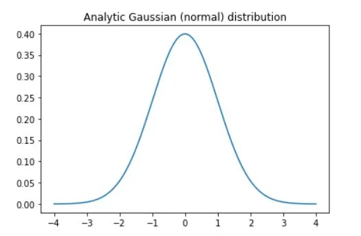
The graph of the Gaussian distribution is characterized by two parameters: the mean (μ) and the standard deviation (σ). The mean represents the average value and serves as the maximum point of the graph, around which the distribution is symmetric. The standard deviation determines the dispersion or spread of the data away from the mean. A small standard deviation results in a steep graph, while a large standard deviation produces a flatter graph.

import matplotlib.pyplot as plt
import numpy as np
import scipy.stats as stats

# number of discretizations
N = 1001

x = np.linspace(-4,4,N)
gausdist = stats.norm.pdf(x)

plt.plot(x,gausdist)
plt.title('Analytic Gaussian (normal) distribution')
plt.show()

print(sum(gausdist))       

Uniform distribution:

Uniform distribution is a fundamental concept in probability theory and statistics, characterized by its simplicity and equal probability for all outcomes. It is a continuous probability distribution that has numerous applications in various fields, including computer simulations, cryptography, and statistical modeling. In this blog post, we will explore the origins of uniform distribution, its characteristics, and its significance in real-world applications.

The concept of uniform distribution dates back to ancient times when the Greek philosopher Aristotle introduced the idea of equiprobability, which states that all outcomes of an event have an equal chance of occurring. This idea was later formalized by French mathematician Pierre-Simon Laplace in the 18th century, who developed the principle of insufficient reason, which asserts that in the absence of any information, all outcomes should be considered equally likely.

import matplotlib.pyplot as plt
import numpy as np
import scipy.stats as stats

# parameters
stretch = 2 # not the variance
shift   = .5
n       = 10000

# create data
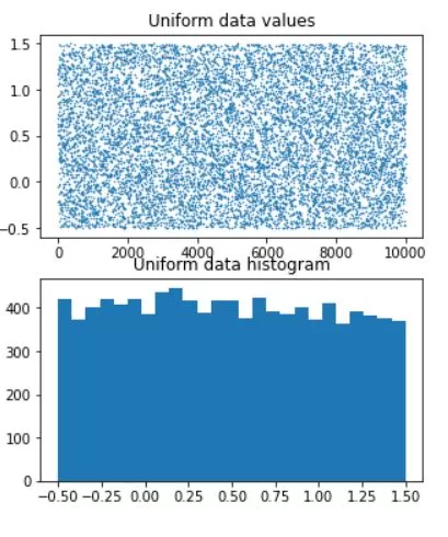
data = stretch*np.random.rand(n) + shift-stretch/2

# plot data
fig,ax = plt.subplots(2,1,figsize=(5,6))

ax[0].plot(data,'.',markersize=1)
ax[0].set_title('Uniform data values')

ax[1].hist(data,25)
ax[1].set_title('Uniform data histogram')

plt.show()

Log-normal distribution:

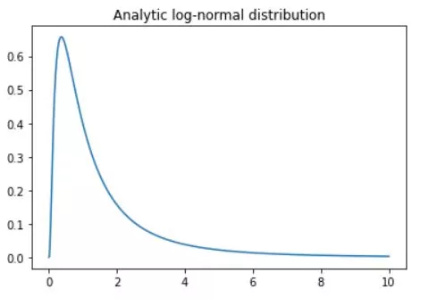
The log-normal distribution, also known as the Galton distribution, is a continuous probability distribution with a normally distributed logarithm. It is a versatile concept in probability theory and statistics, characterized by its skewed distribution, low mean values, large variance, and all-positive values. In this blog post, we will delve into the origins of log-normal distribution, its characteristics, and its significance in real-world applications, particularly in finance.
The log-normal distribution was first introduced by Francis Galton, a British scientist, and cousin of Charles Darwin, in the late 19th century. Galton's work on the distribution was inspired by his studies on heredity and natural selection. He observed that many natural phenomena, such as the size of biological organisms and the distribution of wealth, exhibited a skewed distribution that could be modeled using the logarithm of a normally distributed random variable.

import matplotlib.pyplot as plt
import numpy as np
import scipy.stats as stats

N = 1001
x = np.linspace(0,10,N)
lognormdist = stats.lognorm.pdf(x,1)

plt.plot(x,lognormdist)
plt.title('Analytic log-normal distribution')
plt.show()

Binomial distribution:

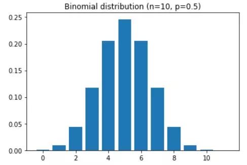
The binomial distribution is a discrete probability distribution that models the number of successes in a fixed number of independent Bernoulli trials with the same probability of success. It is a fundamental concept in probability theory and statistics, with numerous applications in various fields, including finance, quality control, and social sciences. In this blog post, we will explore the characteristics of binomial distribution and its significance in real-world applications.

A good example of binomial distribution is the probability of K heads in N coin tosses, given a probability of p heads (e.g., .5 is a fair coin).

import matplotlib.pyplot as plt
import numpy as np
import scipy.stats as stats

n = 10 # number on coin tosses
p = .5 # probability of heads

x = range(n+2)
bindist = stats.binom.pmf(x,n,p)

plt.bar(x,bindist)
plt.title('Binomial distribution (n=%s, p=%g)'%(n,p))
plt.show()

F distribution:

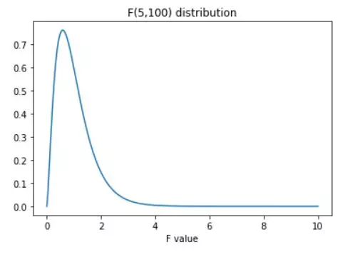
The F distribution, also known as the Snedecor's F distribution or the Fisher-Snedecor distribution, is a continuous probability distribution that arises in the context of hypothesis testing and analysis of variance (ANOVA). It is a fundamental concept in statistics, with numerous applications in various fields, including finance, quality control, and social sciences.
The F-distribution is a way of obtaining the probabilities of specific sets of events. The F-statistic is often used to evaluate the significant difference of a theoretical data models.

import matplotlib.pyplot as plt
import numpy as np
import scipy.stats as stats

# parameters
num_df = 5   # numerator degrees of freedom
den_df = 100 # denominator df

# values to evaluate 
x = np.linspace(0,10,10001)

# the distribution
fdist = stats.f.pdf(x,num_df,den_df)

plt.plot(x,fdist)
plt.title(f'F({num_df},{den_df}) distribution')
plt.xlabel('F value')
plt.show()

T distribution:

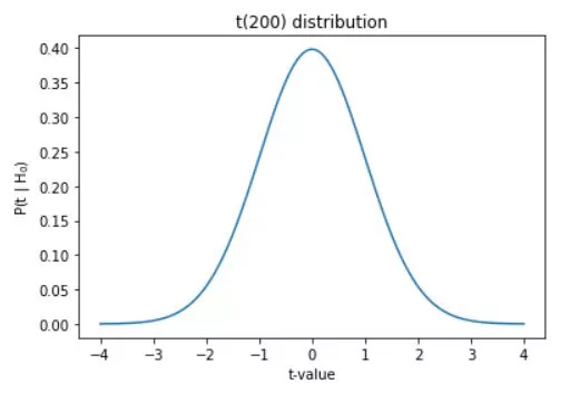
The t distribution, also known as the Student's t distribution, is a continuous probability distribution that plays a crucial role in hypothesis testing and confidence interval estimation, particularly when dealing with small sample sizes. Developed by William Sealy Gosset under the pseudonym "Student," the t distribution is a fundamental concept in statistics, with numerous applications in various fields, including finance, quality control, and social sciences.

import matplotlib.pyplot as plt
import numpy as np
import scipy.stats as stats

x  = np.linspace(-4,4,1001)
df = 200
t  = stats.t.pdf(x,df)

plt.plot(x,t)
plt.xlabel('t-value')
plt.ylabel('P(t | H$_0$)')
plt.title('t(%g) distribution'%df)
plt.show()

Checking distribution type:

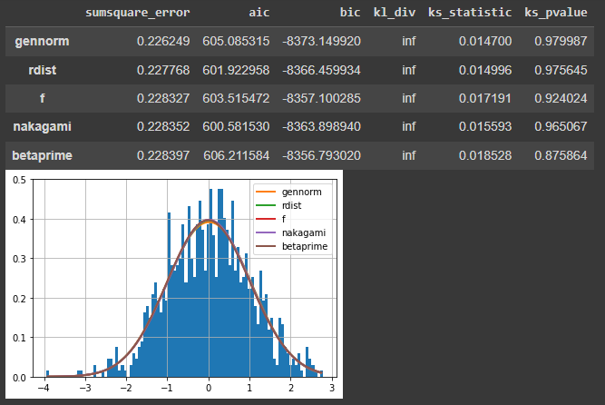
You can check distribution type using Fitter library (don't forget to pip install it) and simple code below. In this example we generate random normal distribution using numpy, Fitter will check your data against different distributions, about 100 at the moment I test my code. If the test takes a long time, you can reduse the number of tested templates - f = Fitter(data, distributions=['gamma', 'rayleigh', 'uniform', 'normal', 'student', 'gennorm']).

from fitter import Fitter
import numpy as np

data = np.random.normal(size=(1000))

f=Fitter(data)
f.fit()
f.summary()