Rank correlation in statistics.
If you're navigating the world of data analysis and want to delve into measuring the strength of relationships in ordinal data, you're in the right place. Kendall Correlation, also known as Kendall's tau coefficient, provides a powerful tool to uncover associations and dependencies in your data. In this guide, we'll walk you through the theory behind Kendall Correlation, explain its calculation and interpretation, and provide practical examples of implementing it in Python. By the end, you'll be equipped with the knowledge and skills to confidently analyze and interpret ordinal data using Kendall Correlation in Python.
Let's dive in and unlock the insights waiting to be discovered!

Python Knowledge Base: Make coding great again.
- Updated:
2026-07-21 by Andrey BRATUS, Senior Data Analyst.
Kendall's rank for correlated data - movie ratings and education level:
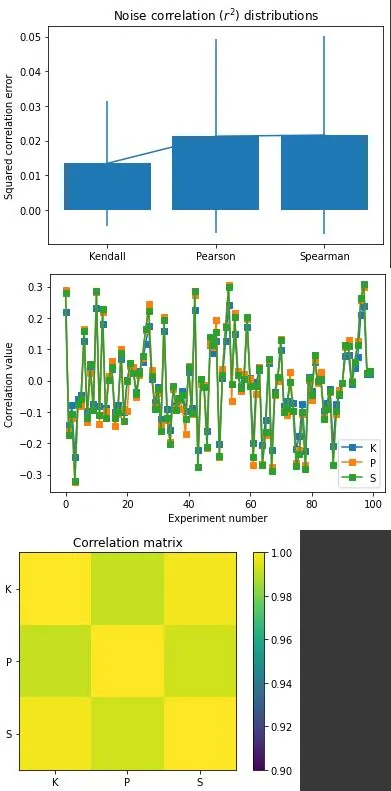
Correlation estimation errors under H0:
Correlation comparison - the graphs:
Real-World Application of Kendall Correlation.
Advantages and Limitations of Kendall Correlation.
Conclusion.
In statistics Kendall's rank correlation produces a distribution-free test of independence and a measure of the strength of ordinal association between two variables.
It is named after Maurice Kendall, who developed it in 1938.
Kendall's tau, like Spearman's rank correlation, is carried
out on the ranks of the data.
The Kendall correlation between two variables will be high when observations have a similar rank between the two variables, and low when observations have a different rank between the two variables.
Spearman's rank correlation is a more widely used measure of rank
correlation because it is much easier to compute than Kendall's tau. The
main advantages of using Kendall's tau are that the distribution of this
statistic has slightly better statistical properties and there is a direct
interpretation of Kendall's tau in terms of probabilities of observing
concordant and discordant pairs. In almost all situations the
values of Spearman's rank correlation and Kendall's tau are very close and
would invariably lead to the same conclusions.
import matplotlib.pyplot as plt
import numpy as np
import scipy.stats as stats

N = 40

# movie ratings
docuRatings = np.random.randint(low=1,high=6,size=N)

# education level (1-4, correlated with docuRatings)
eduLevel = np.ceil( (docuRatings + np.random.randint(low=1,high=5,size=N) )/9 * 4 )

# compute the correlations
cr = [0,0,0]
cr[0] = stats.kendalltau(eduLevel,docuRatings)[0]
cr[1] = stats.pearsonr(eduLevel,docuRatings)[0]
cr[2] = stats.spearmanr(eduLevel,docuRatings)[0]

# round for convenience
cr = np.round(cr,4)


# plot the data
plt.plot(eduLevel+np.random.randn(N)/30,docuRatings+np.random.randn(N)/30,'ks',markersize=10,markerfacecolor=[0,0,0,.25])
plt.xticks(np.arange(4)+1)
plt.yticks(np.arange(5)+1)
plt.xlabel('Education level')
plt.ylabel('Documentary ratings')
plt.grid()
plt.title('$r_k$ = %g, $r_p$=%g, $r_s$=%g'%(cr[0],cr[1],cr[2]))

plt.show()
numExprs = 1000
nValues = 50
nCategories = 6
c = np.zeros((numExprs,3))
for i in range(numExprs):
# create data
x = np.random.randint(low=0,high=nCategories,size=nValues)
y = np.random.randint(low=0,high=nCategories,size=nValues)
# store correlations
c[i,:] = [ stats.kendalltau(x,y)[0],
stats.pearsonr(x,y)[0],
stats.spearmanr(x,y)[0] ]
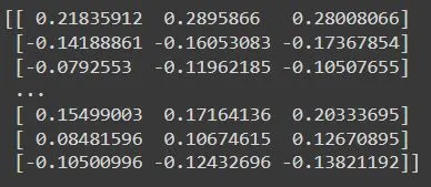
print(c)
plt.bar(range(3),np.mean(c**2,axis=0))
plt.errorbar(range(3),np.mean(c**2,axis=0),yerr=np.std(c**2,ddof=1,axis=0))
plt.xticks(range(3),('Kendall','Pearson','Spearman'))
plt.ylabel('Squared correlation error')
plt.title('Noise correlation ($r^2$) distributions')
plt.show()


plt.plot(c[:100,:],'s-')
plt.xlabel('Experiment number')
plt.ylabel('Correlation value')
plt.legend(('K','P','S'))
plt.show()


plt.imshow(np.corrcoef(c.T),vmin=.9,vmax=1)
plt.xticks(range(3),['K','P','S'])
plt.yticks(range(3),('K','P','S'))
plt.colorbar()
plt.title('Correlation matrix')
plt.show()
In finance, Kendall Correlation is widely used for analyzing portfolio diversification, identifying potential risks, and calculating asset pricing models. Its robustness against outliers and non-normality makes it a good choice for financial data analysis.
In marketing, Kendall Correlation helps in identifying correlations between advertising strategies and consumer behaviour. Marketers can analyze which marketing strategies are more effective and can plan their campaigns accordingly.
In climate research, Kendall Correlation is used for studying relationships between different variables like temperature, humidity, and precipitation. It helps in identifying patterns and forecasting extreme weather conditions.
Advantages of using Kendall Correlation includes the ability to handle both continuous and ordinal data and is less sensitive to outliers. Kendall Correlation measures association rather than causation, preventing a wrong interpretation of the relationship. Additionally, it is robust to assumptions of normality, making it a preferred choice when the variables' distributions are unknown.
On the other hand, the Limitations of Kendall Correlation include its unsuitability to measure the strength of linear relationships and has less power than other correlation measures for small sample sizes. Furthermore, Kendall Correlation is not appropriate for measuring the association between variables with a non-monotonic relationship.
In comparison with other correlation measures, Kendall Correlation performs well when dealing with a small sample size and is not influenced by extreme values. However, it may be underpowered when the data has a normal distribution and a linear association.
To sum up, Kendall Correlation is a vital tool in data analysis. It helps to understand the strength of a relationship between variables. To derive correct insights, it is important to use it with due diligence. Happy analyzing!