Leveraging Python for the Law of Large Numbers in Data Science.

Theoretical Framework.

If you've ever taken a statistics course, you might be familiar with the concept of the Probability Distribution. In simple terms, the probability distribution is just a function that maps a range of possible events to their associated probabilities. Probability distributions exist all around us, from the distribution of heights in a population to the distribution of grades in a class.

When working with probability distributions, it's often useful to have some way of summarizing the data. This is where the Sample Mean and Population Mean come in. The Sample Mean is simply the average of a set of scores, while the Population Mean is the average of all possible scores in a population. These summary measures allow us to quickly get a sense of the underlying distribution.

So where do LLNs come in? Well, LLNs provide a way of predicting the behavior of a distribution based on a sample of data. The basic idea is that as the sample size increases, the sample mean will tend to converge to the population mean. This means that we can use a large enough sample to make highly accurate predictions about the behavior of the underlying distribution.

When working with LLNs, it's important to keep in mind the assumptions that underlie the method. Specifically, LLNs assume that the data are independent and identically distributed (IID). This means that each data point is drawn from the same distribution and that the data points are not influenced by each other.

Overall, LLNs provide a powerful tool for working with probability distributions. By allowing us to make accurate predictions based on a sample of data, LLNs can help us to better understand and analyze complex phenomena in the world around us.

Moving Forward with LLN.

The law of large numbers has a very central role in probability and statistics. LLN or the law of large numbers is a theorem that depicts the result of performing the same experiment a large number of times. The average of the results obtained from a large number of trials should be close to the expected value and will tend to become closer to the expected value as more attempts are performed. The law of large numbers guarantees stable long-term results for the averages of some random events.
The Law of Large Numbers is not to be mistaken with the Law of Averages, which states that the distribution of outcomes in a sample (large or small) reflects the distribution of outcomes of the population.

Example: rolling a die:

Expected value (also known as EV or expectation) is a long-run average value of random variables. It also indicates the probability-weighted average of all possible values.
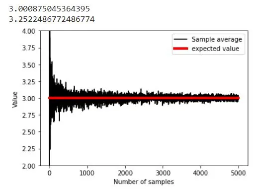
In following examle of rolling a die we visualise sample average vs expected value dependency. IMPORTANT: this step does not show LLN yet !!!

import matplotlib.pyplot as plt
import numpy as np


# die probabilities (weighted)
f1 = 2/8
f2 = 2/8
f3 = 1/8
f4 = 1/8
f5 = 1/8
f6 = 1/8

# confirm sum to 1
print(f1+f2+f3+f4+f5+f6)

# expected value
expval = 1*f1 + 2*f2 + 3*f3 + 4*f4 + 5*f5 + 6*f6

# generate "population"
population = [ 1, 1, 2, 2, 3, 4, 5, 6 ]
for i in range(20):
    population = np.hstack((population,population))

nPop = len(population)

# draw sample of 8 rolls
sample = np.random.choice(population,8)

## experiment: draw larger and larger samples

k = 5000  # maximum number of samples
sampleAve = np.zeros(k)

for i in range(k):
    idx = np.floor(np.random.rand(i+1)*nPop)
    sampleAve[i] = np.mean( population[idx.astype(int)] )


plt.plot(sampleAve,'k')
plt.plot([1,k],[expval,expval],'r',linewidth=4)
plt.xlabel('Number of samples')
plt.ylabel('Value')
plt.ylim([expval-1, expval+1])
plt.legend(('Sample average','expected value'))

# mean of samples converges to population estimate quickly:
print( np.mean(sampleAve) )
print( np.mean(sampleAve[:9]) )

LLN - computing sample means vs expected value:

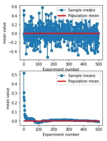
IMPORTANT: this is LLN demonstration !!!

# generate population data with known mean
populationN = 1000000
population = np.random.randn(populationN)
population = population - np.mean(population)  # demean


# get means of samples
samplesize   = 30
numberOfExps = 500
samplemeans  = np.zeros(numberOfExps)

for expi in range(numberOfExps):
    # get a sample and compute its mean
    sampleidx = np.random.randint(0,populationN,samplesize)
    samplemeans[expi] = np.mean(population[ sampleidx ])


# show the results!
fig,ax = plt.subplots(2,1,figsize=(4,6))
ax[0].plot(samplemeans,'s-')
ax[0].plot([0,numberOfExps],[np.mean(population),np.mean(population)],'r',linewidth=3)
ax[0].set_xlabel('Experiment number')
ax[0].set_ylabel('mean value')
ax[0].legend(('Sample means','Population mean'))

ax[1].plot(np.cumsum(samplemeans) / np.arange(1,numberOfExps+1),'s-')
ax[1].plot([0,numberOfExps],[np.mean(population),np.mean(population)],'r',linewidth=3)
ax[1].set_xlabel('Experiment number')
ax[1].set_ylabel('mean value')
ax[1].legend(('Sample means','Population mean'))

plt.show()

Scope and Limitations of LLNs.

As much as we would like to rely on LLNs for our statistical analysis, there are a few limitations to its application. Firstly, LLNs assume that there are a large number of identical trials, however, in real-world scenarios, this might not be the case. Additionally, LLNs cannot account for outliers or extreme values, which can skew the results.

However, we can still apply LLNs in situations where the limitations are not significant. For example, LLNs are very useful in situations where we have a small sample size but can create a large number of identical trials through simulation. LLNs are also effective in identifying trends and patterns in data sets.

To overcome the limitations of LLNs, there are other statistical methods available that can be used in combination with LLNs such as bootstrapping and the jackknife method. These methods can help identify outliers and extreme values in the data set, which in turn can be used to refine the LLN analysis.

LLNs in Real-world Scenarios.

Now that we have a clear idea about what LLNs are, let us explore their real-world applications. LLNs have many purposes in finance and gambling. In finance, LLNs play a crucial role in analyzing the stock market and assessing risks. In gambling, LLNs help in predicting the outcome of games and improving the odds of winning.

LLNs also have a significant role in healthcare and clinical trials. With the increasing demand for new drugs and treatments, LLNs come into play when selecting sample sizes for testing. Accurate sample sizes determine the true effects of a trial and the potential risks associated with it.

LLNs are equally important in data analysis. They help in finding the mean of a population with high accuracy and lower the uncertainty associated with the sample. Without LLNs, the accuracy of most statistical models would be questionable.

In conclusion, LLNs play a critical role in various fields, including finance, healthcare, and data analysis. Its applications are vast, and it's unlikely that its prominence will diminish any time soon.

Conclusion.

So there you have it - the Law of Large Numbers with Python. We've seen how LLNs play a crucial role in understanding probability distribution and how we can use CLT to explain it even better. We've also explored the limitations and scope of LLNs, as well as its real-world applications. Python libraries like Numpy, SciPy, and Matplotlib make it easy to work with LLNs. Knowing the importance of LLNs in statistical analysis and its future scope is crucial for any budding data scientist. So go ahead, try it out for yourself, and see the wonders of LLNs unfold.