Quick dive into non-Pearson Data Analysis.
Do you want to learn how to calculate Spearman correlation and Fisher-Z transformations using Python? Mastering these techniques can help you to better analyze and understand your data. With this tutorial, you will gain a comprehensive understanding of Spearman Correlation & Fisher-Z and how to use Python to calculate them accurately.

Python Knowledge Base: Make coding great again.
- Updated:
2026-07-23 by Andrey BRATUS, Senior Data Analyst.
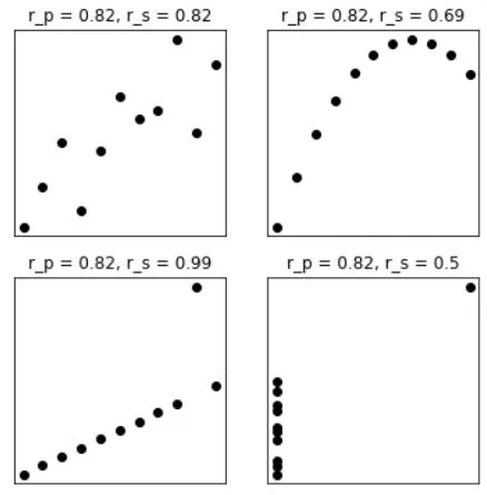
Anscobe's quartet visualization with correlations:
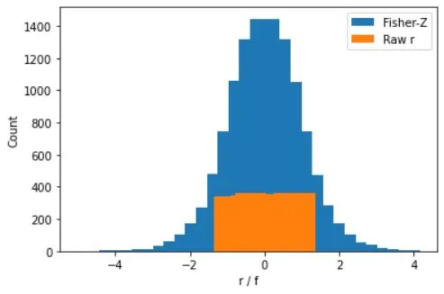
Fisher-Z transformation:
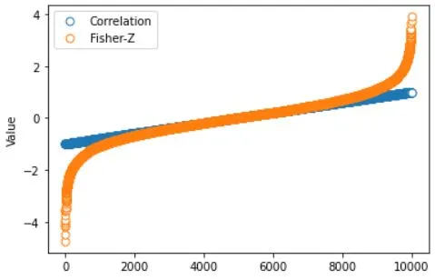
Correlation VS Fisher-Z:
Benefits and limitations of Spearman Correlation and Fisher-Z Transformation.
Correlation plays a critical role in analyzing the relationship between variables, primarily in statistics and data science. It helps in identifying patterns and trends, understanding the strength and direction of the relationship, and predicting future outcomes. There are different types of correlations, such as Pearson, Spearman, and Kendall.
Classical Pearson correlation has limitations as high sensitivity to outliers and tends to inftale or deflate nonlinear relationships, i e appropriate for normal data. Unlike Pearson’s correlation, there is no requirement of normality and hence it
is a nonparametric statistic.
To understand Spearman’s correlation it is necessary to know what a monotonic
function is. A monotonic function is one that either never increases or never decreases
as its independent variable increases.Spearman’s correlation works by calculating Pearson’s correlation on the ranked
values of this data.
Intuition behind Spearman’s correlation values - the same as classical Pearson correlation.
* .00-.19 “very weak”
* .20-.39 “weak”
* .40-.59 “moderate”
* .60-.79 “strong”
* .80-1.0 “very strong”
Fisher's r to z transformation is a statistical method that converts a Pearson product-moment correlation coefficient to a standardized z score in order to assess whether the correlation is statistically different from zero.
import matplotlib.pyplot as plt
import numpy as np
import scipy.stats as stats


anscombe = np.array([
     # series 1     series 2      series 3       series 4
    [10,  8.04,    10,  9.14,    10,  7.46,      8,  6.58, ],
    [ 8,  6.95,     8,  8.14,     8,  6.77,      8,  5.76, ],
    [13,  7.58,    13,  8.76,    13, 12.74,      8,  7.71, ],
    [ 9,  8.81,     9,  8.77,     9,  7.11,      8,  8.84, ],
    [11,  8.33,    11,  9.26,    11,  7.81,      8,  8.47, ],
    [14,  9.96,    14,  8.10,    14,  8.84,      8,  7.04, ],
    [ 6,  7.24,     6,  6.13,     6,  6.08,      8,  5.25, ],
    [ 4,  4.26,     4,  3.10,     4,  5.39,      8,  5.56, ],
    [12, 10.84,    12,  9.13,    12,  8.15,      8,  7.91, ],
    [ 7,  4.82,     7,  7.26,     7,  6.42,      8,  6.89, ],
    [ 5,  5.68,     5,  4.74,     5,  5.73,     19, 12.50, ]
    ])


# plot and compute correlations
fig,ax = plt.subplots(2,2,figsize=(6,6))
ax = ax.ravel()

for i in range(4):
    ax[i].plot(anscombe[:,i*2],anscombe[:,i*2+1],'ko')
    ax[i].set_xticks([])
    ax[i].set_yticks([])
    corr_p = stats.pearsonr(anscombe[:,i*2],anscombe[:,i*2+1])[0]
    corr_s = stats.spearmanr(anscombe[:,i*2],anscombe[:,i*2+1])[0]
    ax[i].set_title('r_p = %g, r_s = %g'%(np.round(corr_p*100)/100,np.round(corr_s*100)/100))

plt.show()
# simulate correlation coefficients
N = 10000
r = 2*np.random.rand(N) - 1

# Fisher-Z
fz = np.arctanh(r)


# overlay the Fisher-Z
y,x = np.histogram(fz,30)
x = (x[1:]+x[0:-1])/2
plt.bar(x,y)

# raw correlations
y,x = np.histogram(r,30)
x = (x[1:]+x[0:-1])/2
plt.bar(x,y)


plt.xlabel('r / f')
plt.ylabel('Count')
plt.legend(('Fisher-Z','Raw r'))

plt.show()
plt.plot(range(N),np.sort(r), 'o',markerfacecolor='w',markersize=7)
plt.plot(range(N),np.sort(fz),'o',markerfacecolor='w',markersize=7)
plt.ylabel('Value')
plt.legend(('Correlation','Fisher-Z'))

# zoom in
# plt.ylim([-.8,.8])
plt.show()
Benefits of Spearman Correlation:
Non-Parametric Analysis: Spearman Correlation is a non-parametric measure, meaning it does not assume that the data follows a specific distribution. This makes it suitable for analyzing variables that may not meet the assumptions of parametric tests like the Pearson Correlation.
Robustness to Outliers: Spearman Correlation is less sensitive to outliers compared to the Pearson Correlation. It is based on ranks rather than actual values, making it more resistant to extreme observations that could distort the correlation measure.
Captures Monotonic Relationships: Spearman Correlation captures monotonic relationships between variables, which means it can detect nonlinear associations that may not be captured by the Pearson Correlation. This makes it particularly useful in analyzing ordinal or skewed data.
Interpretability: The Spearman Correlation coefficient ranges between -1 and 1, providing a measure of the strength and direction of the relationship between variables. This interpretability allows for easy comparison and understanding of the correlation magnitude.
Benefits of Fisher-Z Transformation:
Stabilization of Correlation Coefficients: The Fisher-Z Transformation is commonly used to stabilize the distribution and standardize the variance of correlation coefficients. This helps when comparing correlation values across studies or when applying further statistical analyses that assume a normal distribution.
Enabling Parametric Analyses: By transforming correlation coefficients using Fisher-Z Transformation, it is possible to perform additional statistical tests, such as hypothesis testing and confidence interval estimation, assuming a normal distribution. This allows for more robust inferential analyses.
Limitations:
Assumes Monotonicity: Spearman Correlation assumes that the relationship between variables is monotonic, meaning that as one variable increases, the other variable consistently increases or decreases. If the relationship between variables is not monotonic, Spearman Correlation may not accurately capture the association.
Discards Magnitude Differences: Both Spearman Correlation and Fisher-Z Transformation focus solely on the ranks or relative positions of the data and do not consider the actual magnitude of the values. This means that they might miss important information related to the strength of the association between variables.
Restricted to Ordinal Data: While Spearman Correlation can be used with both ordinal and interval data, it is less efficient when applied to interval-scaled variables. In such cases, Pearson Correlation may provide more accurate results.
Sensitivity to Ties: Spearman Correlation may be sensitive to tied values within the dataset. When ties exist, the calculation of ranks affects the precision of the correlation estimate. Proper handling of tied values is crucial to ensure accurate results.
It is important to consider these benefits and limitations when choosing and interpreting the results obtained from Spearman Correlation and Fisher-Z Transformation in statistical analyses.