Unlock the Power of Dispersion Calculation in Python.

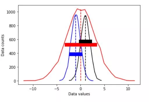
Statistical calculation that allows us to tell how far apart our data is spread is called dispersion.

Variance is a simple measure of dispersion. Variance measures how far each number in the dataset from the mean. To compute variance first, calculate the mean and squared deviations from a mean.
Standard deviation is a squared root of the variance to get original values. Low standard deviation indicates data points close to mean.

# import libraries
import matplotlib.pyplot as plt
import numpy as np

## create some data distributions

# the distributions
N = 10001   # number of data points
nbins = 30  # number of histogram bins

d1 = np.random.randn(N) - 1
d2 = 3*np.random.randn(N)
d3 = np.random.randn(N) + 1

# need their histograms
y1,x1 = np.histogram(d1,nbins)
x1 = (x1[1:]+x1[:-1])/2

y2,x2 = np.histogram(d2,nbins)
x2 = (x2[1:]+x2[:-1])/2

y3,x3 = np.histogram(d3,nbins)
x3 = (x3[1:]+x3[:-1])/2

meanval = 10.2
stdval  = 7.5
numsamp = 123

np.random.normal(meanval,stdval,numsamp)

# compute the means
mean_d1 = sum(d1) / len(d1)
mean_d2 = np.mean(d2)
mean_d3 = np.mean(d3)

## now for the standard deviation

# initialize
stds = np.zeros(3)

# compute standard deviations
stds[0] = np.std(d1,ddof=1)
stds[1] = np.std(d2,ddof=1)
stds[2] = np.std(d3,ddof=1)


# same plot as earlier
plt.plot(x1,y1,'b', x2,y2,'r', x3,y3,'k')
plt.plot([mean_d1,mean_d1],[0,max(y1)],'b--', [mean_d2,mean_d2],[0,max(y2)],'r--',[mean_d3,mean_d3],[0,max(y3)],'k--')

# now add stds
plt.plot([mean_d1-stds[0],mean_d1+stds[0]],[.4*max(y1),.4*max(y1)],'b',linewidth=10)
plt.plot([mean_d2-stds[1],mean_d2+stds[1]],[.5*max(y2),.5*max(y2)],'r',linewidth=10)
plt.plot([mean_d3-stds[2],mean_d3+stds[2]],[.6*max(y3),.6*max(y3)],'k',linewidth=10)

plt.xlabel('Data values')
plt.ylabel('Data counts')
plt.show()   

Get ready to explore the diverse landscape of variability and its impact on your data-driven projects.
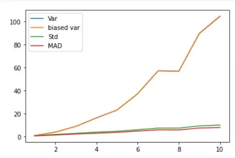
Variance is a fundamental concept in statistics that measures the dispersion or spread of data points in a dataset. It helps us understand the degree of variability within the data, which is crucial for making informed decisions and drawing accurate conclusions. In this section, we'll delve into the importance of variance and its role in statistical analysis.

Mean absolute deviation of given data poins is the average distance between each data value and the mean. Mean absolute deviation is a way to describe variation in a data and gives us understanding of how "spread out" the values in a data set are.

variances = np.arange(1,11)
N = 300

varmeasures = np.zeros((4,len(variances)))

for i in range(len(variances)):
    
    # create data and mean-center
    data = np.random.randn(N) * variances[i]
    datacent = data - np.mean(data)
    
    # variance
    varmeasures[0,i] = sum(datacent**2) / (N-1)
    
    # "biased" variance
    varmeasures[1,i] = sum(datacent**2) / N
    
    # standard deviation
    varmeasures[2,i] = np.sqrt( sum(datacent**2) / (N-1) )
    
    # MAD (mean absolute difference)
    varmeasures[3,i] = sum(abs(datacent)) / (N-1)
    

# show them!
plt.plot(variances,varmeasures.T)
plt.legend(('Var','biased var','Std','MAD'))
plt.show() 

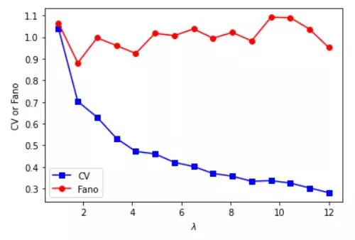
Fano factor is a measure of the dispersion of a probability distribution of a Fano noise and might be considered to be an intensity independent measure of variability.

The coefficient of variation (CV) is a statistical measure of the dispersion of data set around the mean. In finance, the coefficient of variation allows investors to determine volatility or risk in comparison to the amount of return expected from investments.

# need positive-valued data (why?)
data = np.random.poisson(3,300)  # "Poisson noise"

fig,ax = plt.subplots(2,1)
ax[0].plot(data,'s')
ax[0].set_title('Poisson noise')

## compute fano factor and CV for a range of lambda parameters

# list of parameters
lambdas = np.linspace(1,12,15)

# initialize output vectors
fano = np.zeros(len(lambdas))
cv   = np.zeros(len(lambdas))

for li in range(len(lambdas)):
    
    # generate new data
    data = np.random.poisson(lambdas[li],1000)
    
    # compute the metrics
    cv[li]   = np.std(data) / np.mean(data) # need ddof=1 here?
    fano[li] = np.var(data) / np.mean(data)


# and plot
plt.plot(lambdas,cv,'bs-')
plt.plot(lambdas,fano,'ro-')
plt.legend(('CV','Fano'))
plt.xlabel('$\lambda$')
plt.ylabel('CV or Fano')
plt.show()

Variance measures play a vital role in various real-world scenarios, from finance and economics to engineering and social sciences. In this section, we'll discuss some practical applications of variance measures, such as risk assessment in investment portfolios, quality control in manufacturing, and understanding income inequality in economics.

Understanding different variance measures in statistics is essential for anyone working with data. By exploring the diverse landscape of variability, you can make more informed decisions, draw accurate conclusions, and enhance your statistical analysis skills. So, dive into the world of variance measures and unlock the power of data-driven insights.