Confidence intervals in statistics.
Welcome to our comprehensive guide on computing confidence intervals with Python. As a powerful tool for statistical analysis, Python offers a practical and efficient approach to calculating confidence intervals, a crucial aspect in the realm of data science and statistics. Whether you're a seasoned or a beginner in the field, our step-by-step guide will help you master the art of computing confidence intervals using Python. Dive into the world of Python statistics and unlock new potentials in your data analysis journey.

Python Knowledge Base: Make coding great again.
- Updated:
2026-07-19 by Andrey BRATUS, Senior Data Analyst.
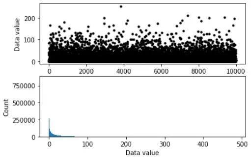
Generating initial data for CI calculation:
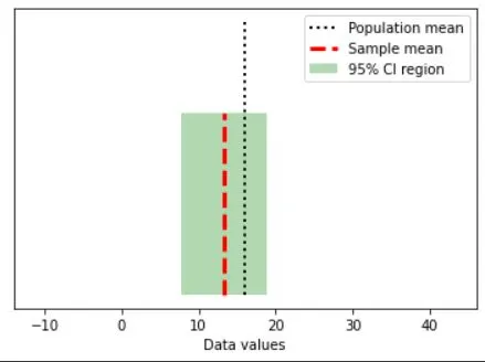
Drawing a random sample with confidence intervals:
Distribution of null hypothesis values:
Empowering Data Analysis with CI.
Conclusion.
A confidence interval (CI) defines the measure of uncertainty in any particular statistic with a certain margin of error.
Or you can say that it is a range of values that’s likely to include a population value with a certain degree of confidence.
As a practical example it tells how confident you can be that the results from a poll or survey reflect what you would expect to find if it were possible to survey the entire population.
Confidence levels are expressed as a percentage ,for example a 95% confidence level.
Where,
x̄: Sample Mean
z: Confidence Coefficient
ơ: Population Standard Deviation
n: Sample Size
The factors affecting the width of the CI include the confidence level, the sample size, and the variability in the sample.
Larger samples produce narrower confidence intervals.
Greater variability in the sample will produce wider confidence intervals.
A higher confidence level will produce a wider confidence interval.
import matplotlib.pyplot as plt
import numpy as np
import scipy.stats as stats
from matplotlib.patches import Polygon

## simulate data

popN = int(1e7)  # lots and LOTS of data!!

# the data (note: non-normal!)
population = (4*np.random.randn(popN))**2

# we can calculate the exact population mean
popMean = np.mean(population)

# let's see it
fig,ax = plt.subplots(2,1,figsize=(6,4))

# only plot every 1000th sample
ax[0].plot(population[::1000],'k.')
ax[0].set_xlabel('Data index')
ax[0].set_ylabel('Data value')

ax[1].hist(population,bins='fd')
ax[1].set_ylabel('Count')
ax[1].set_xlabel('Data value')
plt.show()
# parameters
samplesize = 40
confidence = 95 # in percent

# compute sample mean
randSamples = np.random.randint(0,popN,samplesize)
samplemean  = np.mean(population[randSamples])
samplestd   = np.std(population[randSamples],ddof=1)

# compute confidence intervals
citmp = (1-confidence/100)/2
confint = samplemean + stats.t.ppf([citmp, 1-citmp],samplesize-1) * samplestd/np.sqrt(samplesize)


# graph everything
fig,ax = plt.subplots(1,1)

y = np.array([ [confint[0],0],[confint[1],0],[confint[1],1],[confint[0],1] ])
p = Polygon(y,facecolor='g',alpha=.3)
ax.add_patch(p)

# now add the lines
ax.plot([popMean,popMean],[0, 1.5],'k:',linewidth=2)
ax.plot([samplemean,samplemean],[0, 1],'r--',linewidth=3)
ax.set_xlim([popMean-30, popMean+30])
ax.set_yticks([])
ax.set_xlabel('Data values')
ax.legend(('Population mean','Sample mean','%g%% CI region'%confidence))
plt.show()
## repeat for large number of samples

# parameters
samplesize = 50
confidence = 95  # in percent
numExperiments = 5000

withinCI = np.zeros(numExperiments)


# part of the CI computation can be done outside the loop
citmp = (1-confidence/100)/2
CI_T  = stats.t.ppf([citmp, 1-citmp],samplesize-1)
sqrtN = np.sqrt(samplesize)

for expi in range(numExperiments):

    # compute sample mean and CI as above
    randSamples = np.random.randint(0,popN,samplesize)
    samplemean  = np.mean(population[randSamples])
    samplestd   = np.std(population[randSamples],ddof=1)
    confint     = samplemean + CI_T * samplestd/sqrtN

    # determine whether the True mean is inside this CI
    if popMean>confint[0] and popMean<=confint[1]:
        withinCI[expi] = 1


print('%g%% of sample C.I.''s contained the true population mean.'%(100*np.mean(withinCI)))
OUT: 91.98% of sample C.I.s contained the true population mean.
In the realm of statistical data analysis, confidence intervals play a crucial role. These a reliable range for an unknown parameter, and Python - a versatile programming language rich in its statistical capacities, makes computing them a breeze.
For anyone, whether a seasoned data analyst or a newbie stepping into Python-driven statistical analysis, understanding and efficiently applying confidence intervals is indispensable. They offer a range of possible values within which an unknown population parameter lies. This range is calculated from a given dataset and holds a specific level of confidence.
In the domain of statistical analysis, confidence intervals represent a credible range where we can expect to find an unknown population parameter. Extracted from a given dataset, confidence intervals express the reliability of estimation, spanning from lower to upper end - within which the parameter is likely to exist. This allows us to form predictions and make accurate, informed decisions.
We've established the significance of confidence intervals and the edge Python provides in computing them. Let's delve into why their symbiosis is so crucial in our data-charged world.
Firstly, reliability of estimation is paramount in data-driven decision making. Confidence intervals give us a range of values, enhancing accuracy. Whether it's predicting future sales with an e-commerce firm, estimating voters turnout for political research, or understanding user behavior in tech companies, confidence intervals provide a reliable foundation for prediction and planning.
In Python, the statistical models for computing confidence intervals are Z-Score and T-distribution methods for larger and smaller samples respectively. There's also bootstrapping, an advanced approach that allows resampling and provides more flexible analyses.
Secondly, Python's proficiency in handling vast datasets significantly reduces the time taken to compute confidence intervals. This means analysts can focus more on drawing insights rather than getting tangled lengthy calculations. Additionally, the Python ecosystem is ever-evolving, resulting in new tools and libraries that enhance computational efficiency and accuracy, such as seaborn for visualization or pyMC3 for probabilistic programming.
Lastly, with Python's wide usage, there is a vibrant global community supporting its users. This means common challenges are addressed swiftly, and new methodologies and tools are shared expediently, making solutions to statistical problems like computing confidence intervals more accessible.
Confidence intervals, an insightful statistical tool, offers reliable prediction ranges. Python, revered for its statistical prowess, allows accessible and efficient calculations. Coupled together they not only simplify tasks for data analysts but also ensure accurate predictions and robust decision-making processes. Whether you are a businessperson wondering about the potential sales range or a scientist estimating a parameter, computing confidence intervals with Python amplifies the depth and width of your understanding.
While diving into this aspect of data analysis, start with understanding your data. Get hands-on with Python libraries, and delve deeper into methods suitable for your tasks. By leveraging Python’s computational capacity and understanding the critical role of confidence intervals, you can maneuver through the vast ocean of data at your fingertips to extract meaningful and insightful pearls of wisdom.
Remember, the magic lies not merely in the numbers crunched but using these numbers to create far-reaching insights. The potential is immense so, harness the power of Python and confidence intervals to realize it!