Sampling variability quick dive.
Unlock the power of Python in understanding the nuances of 'Sampling Variability'. This comprehensive guide is your gateway to mastering this vital statistical concept, using Python's robust data science libraries. Whether you're a novice or a seasoned data analyst, we'll help you navigate the complexities of sampling variability with ease and precision.

Python Knowledge Base: Make coding great again.
- Updated:
2026-07-24 by Andrey BRATUS, Senior Data Analyst.
Types of Sampling Variability.
Measures of Sampling Variability.
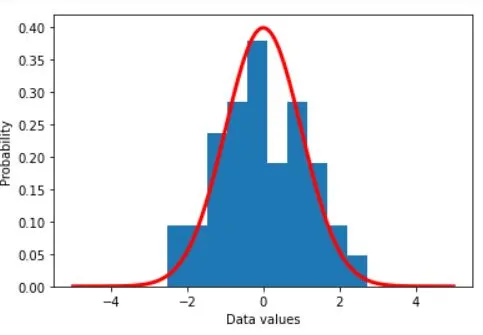
Theoretical distribution (population) and experiment data (sample):
Show the mean of samples of a known distribution:
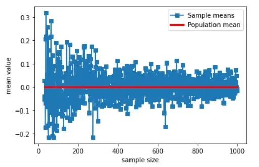
Sample means VS sample sizes:
Confidence Interval.
Conclusion.
Are you tired of encountering sample data that looks vastly different from what you predicted? That's sampling variability for you! Sampling variability refers to the fluctuation of statistics when different samples are taken from the same population. Understanding it is key to making accurate predictions and minimizing errors.
Now, you may be thinking, "How is this relevant to me?" Let's say you want to conduct a survey on the popularity of a new product. You choose a sample size that you think is representative of the population. However, if you don't account for sampling variability, your results may not reflect the true popularity of the product.
To make things more relatable, let's consider an analogy. You're at a restaurant and the first bite of food you take is absolutely delicious. However, each subsequent bite tastes slightly different. Sampling variability is like the inconsistency in quality between each bite, despite coming from the same dish.
Stay tuned to learn more about the types of sampling variability, measures of variation, and how to simulate it through Python!
Sampling variability refers to the natural variation that occurs due to taking a limited sample from a larger population. Understanding this variability is crucial in statistical analysis as it helps to avoid incorrect interpretations. There are three types of sampling variability: systematic sampling variability, random sampling variability, and cluster sampling variability.
Systematic sampling variability arises when the sample is chosen according to a certain pattern in the population. For example, if a survey is conducted by only selecting every third person, it would be subject to systematic sampling variability.
Random sampling variability, on the other hand, occurs when the sample is chosen randomly from the population. This type of variability is often seen as the most accurate way of obtaining a sample that represents the population.
Lastly, cluster sampling variability is observed when the population is grouped into clusters or subgroups, and samples are taken from each cluster. This type of variability is usually used in cases where the population is heterogeneous or dispersed.
Understanding the different types of sampling variability and their impact is necessary in statistical analysis. In the following sections, we will discuss measures of sampling variability, simulation of sampling variability using Python, the Central Limit Theorem and Confidence Intervals.
When it comes to measuring sampling variability, there are three key measures that every data analyst should be familiar with - standard deviation, variance, and coefficient of variation.
Standard deviation is a measure of how spread out a set of data is from its mean. It tells us how much variation there is in a sample, and the larger the standard deviation, the more spread out the data is. Variance is simply the square of the standard deviation, and it's often used in further statistical analyses.
The coefficient of variation, on the other hand, is a relative measure of variability. It's calculated by dividing the standard deviation by the mean, and it's expressed as a percentage. This measure is useful when you want to compare the variability of different datasets that have different scales or units.
Understandably, measuring sampling variability is an essential aspect of data analysis. By using these measures, you can describe and interpret the variability of your data more accurately, which is essential for making informed decisions.
import matplotlib.pyplot as plt
import numpy as np
import scipy.stats as stats

## a theoretical normal distribution
x = np.linspace(-5,5,10101)
theoNormDist = stats.norm.pdf(x)
# (normalize to pdf)
# theoNormDist = theoNormDist*np.mean(np.diff(x))

# now for our experiment
numSamples = 40

# initialize
sampledata = np.zeros(numSamples)

# run the experiment!
for expi in range(numSamples):
    sampledata[expi] = np.random.randn()


# show the results
plt.hist(sampledata,density=True)
plt.plot(x,theoNormDist,'r',linewidth=3)
plt.xlabel('Data values')
plt.ylabel('Probability')
plt.show()
# generate population data with known mean
populationN = 1000000
population  = np.random.randn(populationN)
population  = population - np.mean(population) # demean

# now we draw a random sample from that population
samplesize = 30

# the random indices to select from the population
sampleidx = np.random.randint(0,populationN,samplesize)
samplemean = np.mean(population[ sampleidx ])

### how does the sample mean compare to the population mean?
print(samplemean)
OUT: -0.050885435985437565
samplesizes = np.arange(30,1000)

samplemeans = np.zeros(len(samplesizes))

for sampi in range(len(samplesizes)):

    # nearly the same code as above
    sampleidx = np.random.randint(0,populationN,samplesizes[sampi])
    samplemeans[sampi] = np.mean(population[ sampleidx ])


# show the results!
plt.plot(samplesizes,samplemeans,'s-')
plt.plot(samplesizes[[0,-1]],[np.mean(population),np.mean(population)],'r',linewidth=3)
plt.xlabel('sample size')
plt.ylabel('mean value')
plt.legend(('Sample means','Population mean'))
plt.show()
Do you know how confident you are in your data? No, we are not asking about your self-esteem. We are talking about the confidence interval. The confidence interval is a range of values that tells us how confident we are that the true value of a population parameter falls between those values.
Why is it even needed? Well, when we work with samples, we only have a limited amount of information that could vary. Therefore, we need some measure of how confident we are in our findings. We use a confidence interval to estimate the true population value based on the sample.
Python offers excellent libraries to calculate confidence intervals, making it a breeze. You can use the `t-interval` function from the `scipy` library to calculate the confidence interval. And there, you have it. You are now more confident in your data than ever before.
In summary, sampling variability is an important concept in statistical inference and requires a thorough understanding. Different types of sampling variability such as systematic, random and cluster were covered. Measures of sampling variability like the standard deviation, variance and coefficient of variation were also detailed. Python can be used to simulate sampling variability, central limit theorem and even calculate confidence interval. By comprehending these topics, one can make informed decisions and conclusions based on data. It's indeed a world full of possibilities!