PMF quick dive.
Discover the captivating world of Probability Mass Functions (PMFs) in Python and embark on a journey to master the art of analyzing discrete probability distributions. With our comprehensive guide, you'll learn how to harness the power of Python to create, manipulate, and visualize PMFs, unlocking valuable insights and enhancing your data-driven decision-making skills.

Python Knowledge Base: Make coding great again.
- Updated:
2026-07-17 by Andrey BRATUS, Senior Data Analyst.
Understanding Probability Distributions.
What is Probability Mass Function?
Properties of Probability Mass Function.
Using Probability Mass Function in Python.
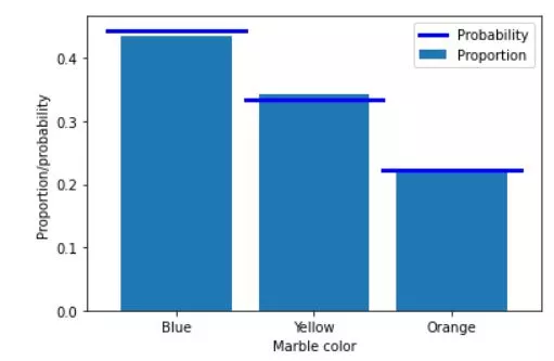
Calculating probability mass function for drawing marbles from a jar:
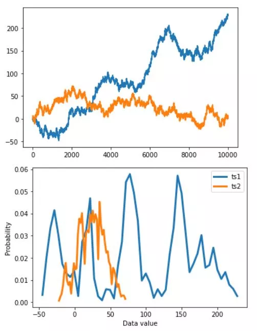
Calculating probability density (technically mass) function:
Real-World Applications of PMF.
Conclusion.
Whether you're a seasoned data scientist or a curious beginner, this tutorial will equip you with the knowledge and tools to conquer the fascinating realm of discrete probability analysis.
Probability distributions refer to the likelihood of occurrence of each possible outcome in an experiment. There are two types of probability distributions, discrete and continuous. Discrete probability distributions are used for experiments where the number of possible outcomes is countable, while continuous probability distributions are used for experiments where the outcomes are real numbers.
Probability density function (PDF) is a continuous probability distribution which describes the probability of a random variable taking a particular value. PDF helps us in identifying the likelihood of different outcomes of a random variable.
Cumulative distribution function (CDF) is another way of representing the probability distribution of a random variable. CDF provides the cumulative probability of random variables up to a certain point. It is useful in calculating probabilities of intervals and percentiles.
Understanding probability distributions is crucial in understanding probability mass functions as they are used for describing the probabilities associated with the values of discrete random variables. By having a basic knowledge of probability distributions, one can easily comprehend probability mass functions and how they can be applied in real-world scenarios.
Probability Mass Function (PMF) is a statistical concept used to define the probability of any discrete random variable. In simpler terms, it calculates the likelihood that a particular variable will take a specific value. Unlike the Continuous Probability Distribution Function (PDF), PMF is used only for discrete variables.
PMF is essential in providing useful information about variables that have a finite set of values. It differs from PDF, which deals with continuous variables. Another difference is that the sum of all probabilities in a PMF is equal to one, whereas in PDF, it is the integral that must be equal to one.
When calculating PMF, the values of the probability for each variable are expressed either in decimals or fractions. In PMF, the probability of a variable is calculated by defining the ratio of possible outcomes of that variable to all possible outcomes.
It can be challenging to understand PMF, but this concept has multiple real-world applications. For example, let's say you're playing a game where the probability of winning or losing is determined by a dice roll. In this game, the PMF can tell you the probability of rolling each value on the dice and help you make informed decisions.
PMF can also help businesses analyze their sales data and make predictions based on the available data. It can also be used in image processing by calculating the probability of the occurrence of pixels in different areas of an image.
In summary, PMF is a crucial concept in statistics and probability theory. Knowing how to calculate it and interpret its results can help you make intelligent decisions and predictions, leading to success in many fields.
Probability Mass Function is widely used in data science for discrete random variables. The properties of Probability Mass Function are crucial in understanding its applications. The domain of a Probability Mass Function represents the set of all possible values of the discrete random variable. The range of Probability Mass Function is a set of non-negative real numbers that sum up to one, which means it represents the probability of the occurrence of each value in the domain.
Probability Axioms specify the essential properties that a probability function must possess. The Probability Mass Function of a Discrete Random Variable with finite or countable infinite set of outcomes assigns each outcome a probability that ranges between 0 and 1, inclusive. The Probability Mass Function is not unique as there may be several valid probability mass functions corresponding to a given discrete random variable.
Understanding these properties is crucial when working with Probability Mass Function in Python. The Probability Mass Function can be used to calculate mean, variance, and standard deviation. Its applications range from analyzing sales data to image processing. It is powerful and versatile and has found applications in several domains, and its use is only expected to increase in the future.
Let's dive into Using Probability Mass Function in Python now. To get started, we need to import the required libraries like NumPy and Matplotlib. Once that is done, creating a Probability Mass Function is as easy as defining an array of possible outcomes and another array of their corresponding probabilities.
With a Probability Mass Function in place, plotting it is just a couple of lines of code away, thanks to the powerful Matplotlib library. You can customize the plot and add labels to make it more visually appealing.
One of the most useful features of a Probability Mass Function is calculating summary statistics like Mean, Variance, and Standard Deviation. And yes, Python can handle it like a pro!
By using Probability Mass Functions in Python, you can automate the process of generating a Probability Mass Function for your data, saving you time and effort. Plus, with Python's user-friendly syntax, you can execute complex operations with ease.
Now that we've seen how powerful Probability Mass Functions can be in Python, let's explore some real-world applications.
The following Python code shows probabilities and proportions calculation for case of drawing marbles of different colors - blue, yellow and orange - out of the box.
import matplotlib.pyplot as plt
import numpy as np

# colored marble counts
blue   = 40
yellow = 30
orange = 20
totalMarbs = blue + yellow + orange

# put them all in a jar
jar = np.hstack((1*np.ones(blue),2*np.ones(yellow),3*np.ones(orange)))

# now we draw 500 marbles (with replacement)
numDraws = 500
drawColors = np.zeros(numDraws)

for drawi in range(numDraws):

    # generate a random integer to draw
    randmarble = int(np.random.rand()*len(jar))

    # store the color of that marble
    drawColors[drawi] = jar[randmarble]

# now we need to know the proportion of colors drawn
propBlue = sum(drawColors==1) / numDraws
propYell = sum(drawColors==2) / numDraws
propOran = sum(drawColors==3) / numDraws


# plot those against the theoretical probability
plt.bar([1,2,3],[ propBlue, propYell, propOran ],label='Proportion')
plt.plot([0.5, 1.5],[blue/totalMarbs, blue/totalMarbs],'b',linewidth=3,label='Probability')
plt.plot([1.5, 2.5],[yellow/totalMarbs,yellow/totalMarbs],'b',linewidth=3)
plt.plot([2.5, 3.5],[orange/totalMarbs,orange/totalMarbs],'b',linewidth=3)

plt.xticks([1,2,3],labels=('Blue','Yellow','Orange'))
plt.xlabel('Marble color')
plt.ylabel('Proportion/probability')
plt.legend()
plt.show()
A probability density function (PDF) differes from probability mass function and associated with continuous rather than discrete random variables.
import matplotlib.pyplot as plt
import numpy as np

# continous signal (technically discrete!)
N = 10004
datats1 = np.cumsum(np.sign(np.random.randn(N)))
datats2 = np.cumsum(np.sign(np.random.randn(N)))

# let's see what they look like
plt.plot(np.arange(N),datats1,linewidth=2)
plt.plot(np.arange(N),datats2,linewidth=2)
plt.show()


# discretize using histograms
nbins = 50

y,x = np.histogram(datats1,nbins)
x1 = (x[1:]+x[:-1])/2
y1 = y/sum(y)

y,x = np.histogram(datats2,nbins)
x2 = (x[1:]+x[:-1])/2
y2 = y/sum(y)


plt.plot(x1,y1, x2,y2,linewidth=3)
plt.legend(('ts1','ts2'))
plt.xlabel('Data value')
plt.ylabel('Probability')
plt.show()
Probability Mass Function in Python has lots of real-world applications, besides its use in theoretical probability calculations. For example, calculating probabilities in gambling games such as poker and blackjack is a common application area, where using PMF is crucial in determining the probabilities of obtaining certain card combinations.
Another notable area of PMF application is analyzing sales data, where PMF can help identify patterns in customer behavior. By analyzing sales data, businesses can make informed decisions such as changing prices, altering product design, and improving customer service.
In image processing, PMF is used to analyze and classify different image components, such as shapes and colors. By using PMF, it is possible to segment images, detect edges and lines, and classify different image regions.
Therefore, PMF is a powerful tool in data science and has many use cases. By using PMF in Python, businesses can make data-driven decisions that lead to improved performance and higher revenue.
In summary, Probability Mass Function in Python is a powerful tool for analyzing and interpreting data in discrete random variables. Its advantages in the field of data science are endless, from calculating probabilities in gambling games to image processing. In Python, it is easy to create, plot and calculate important statistics using the Probability Mass Function. As data science continues to evolve, Probability Mass Function will continue to be a crucial tool for data analysis. So, keep exploring and using Probability Mass Function for all your data science needs!