Python Techniques for Flawless Central Tendency Analysis.

In a world of statistics, a measure of central tendency is a central/typical value for a probability distribution. In everyday life these central/typical values are often called averages.
Measures of central tendency serve to find the middle of a data set. The 3 most common metrics of central tendency are the mean, median and mode.
- Mean: the sum of all values divided by the total number of values.
- Median: the middle number in an ordered data set.
- Mode: the most frequent value of a dataset.

Embark on this enlightening journey and transform your understanding of central tendencies, empowering you to make data-driven decisions with confidence and precision.

Computing the means:

By distilling complex values into a single representative figure, calculating the mean pushes the boundaries of statistical understanding, enabling both professionals and enthusiasts to grasp data-driven insights and make informed decisions.
The arithmetic mean is the sum of all values divided by the total number of values and it’s the most commonly used measure of central tendency. The mean can only be used on interval and ratio levels of measurement because it requires equal spacing between adjacent values or scores in the scale.

# import libraries
import matplotlib.pyplot as plt
import numpy as np
import scipy.stats as stats

# the distributions
N = 10001   # number of data points
nbins = 30  # number of histogram bins

d1 = np.random.randn(N) - 1
d2 = 3*np.random.randn(N)
d3 = np.random.randn(N) + 1

# need their histograms
y1,x1 = np.histogram(d1,nbins)
x1 = (x1[1:]+x1[:-1])/2

y2,x2 = np.histogram(d2,nbins)
x2 = (x2[1:]+x2[:-1])/2

y3,x3 = np.histogram(d3,nbins)
x3 = (x3[1:]+x3[:-1])/2


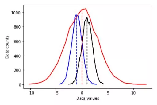
# plot them
plt.plot(x1,y1,'b')
plt.plot(x2,y2,'r')
plt.plot(x3,y3,'k') 

# compute the means
mean_d1 = sum(d1) / len(d1)
mean_d2 = np.mean(d2)
mean_d3 = np.mean(d3)

# plot them
plt.plot(x1,y1,'b', x2,y2,'r', x3,y3,'k')
plt.plot([mean_d1,mean_d1],[0,max(y1)],'b--')
plt.plot([mean_d2,mean_d2],[0,max(y2)],'r--')
plt.plot([mean_d3,mean_d3],[0,max(y3)],'k--')

plt.xlabel('Data values')
plt.ylabel('Data counts')
plt.show()     

Computing the median:

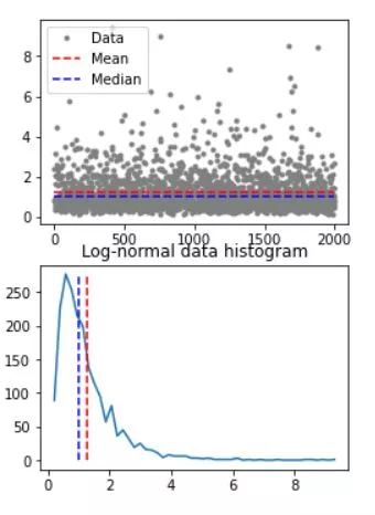
As a robust measure of central tendency, the median skillfully navigates through potential outliers, bringing forth genuine insights and steering us toward sound decision-making. To compute the median, you must first arrange the data in numerical order and identify the middle value. If there are an odd number of values, the median is simply the middle value. If there are an even number of values, you must take the average of the two middle values. The median is useful because it is less sensitive to extreme values than the mean, making it a better representation of the "typical" value in a dataset.
The median can only be used on data that can be ordered – that is, from ordinal, interval and ratio levels of measurement.

# create a log-normal distribution
shift   = 0
stretch = .7
n       = 2000
nbins   = 50

# generate data
data = stretch*np.random.randn(n) + shift
data = np.exp( data )

# and its histogram
y,x = np.histogram(data,nbins)
x = (x[:-1]+x[1:])/2

# compute mean and median
datamean = np.mean(data)
datamedian = np.median(data)


# plot data
fig,ax = plt.subplots(2,1,figsize=(4,6))
ax[0].plot(data,'.',color=[.5,.5,.5],label='Data')
ax[0].plot([1,n],[datamean,datamean],'r--',label='Mean')
ax[0].plot([1,n],[datamedian,datamedian],'b--',label='Median')
ax[0].legend()

ax[1].plot(x,y)
ax[1].plot([datamean,datamean],[0,max(y)],'r--')
ax[1].plot([datamedian,datamedian],[0,max(y)],'b--')
ax[1].set_title('Log-normal data histogram')
plt.show()

Computing the mode:

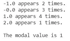
When working with a set of data, it's often helpful to identify the most frequently occurring value, or mode. This is an important statistic that can provide valuable insights into the distribution of the data. To compute the mode, you can simply count the number of times each value appears in the dataset and identify the value with the highest frequency. The mode can be used for any level of measurement, but it’s most meaningful for nominal and ordinal levels.

## mode

data = np.round(np.random.randn(10))

uniq_data = np.unique(data)
for i in range(len(uniq_data)):
    print(f'{uniq_data[i]} appears {sum(data==uniq_data[i])} times.')

print(' ')
print('The modal value is %g'%stats.mode(data)[0][0])