Demystifying Confidence Intervals with Python Bootstrapping.

Confidence Intervals (CI) are a range of values that we construct to estimate a population parameter (e.g. the mean or proportion). They are essential for making informed decisions based on the results of our data analyses.

Classical methods of constructing CIs, such as the t-test and z-test, have been the go-to statistical tools for ages. But like all good things, they too have certain limitations. For instance, they assume a normal distribution of the data, which is not always the case in real-world scenarios. The classical methods can also be biased when dealing with small sample sizes or non-normal distributions.

Bootstrapping is a statistical method or procedure that resamples a single dataset to create many new simulated samples.
Bootstrapping is sometimes called a resample with replacement method.
Bootstrapping VS analytical method for calculating confidence intervals.

PROS/Advantages:
- Can be calculated for any kinds of parameters - mean, variance, correlation, median, etc...
- Very handy for limited data, small number of experiments.
- Not based on assumptions of normality.

CONS/Disadvantages:
- Provides slightly different results for each calculation.
- Time consuming for large datasets.
- There is an assumption that a given sample has a good representation of the true population.

The code below gives an example of calculation confidence intervals using bootstrapping and compares results with analytical method.

Generating initial data for CI calculation:

import matplotlib.pyplot as plt
import numpy as np
import scipy.stats as stats
from matplotlib.patches import Polygon

## simulate data

popN = int(1e7)  # lots and LOTS of data!!

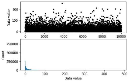
# the data (note: non-normal!)
population = (4*np.random.randn(popN))**2

# we can calculate the exact population mean
popMean = np.mean(population)

# let's see it
fig,ax = plt.subplots(2,1,figsize=(6,4))

# only plot every 1000th sample
ax[0].plot(population[::1000],'k.')
ax[0].set_xlabel('Data index')
ax[0].set_ylabel('Data value')

ax[1].hist(population,bins='fd')
ax[1].set_ylabel('Count')
ax[1].set_xlabel('Data value')
plt.show()

Drawing a random sample with confidence intervals - bootstrapping:

# parameters
samplesize = 40
confidence = 95 # in percent

# compute sample mean
randSamples = np.random.randint(0,popN,samplesize)
sampledata  = population[randSamples]
samplemean  = np.mean(population[randSamples])
samplestd   = np.std(population[randSamples]) # used later for analytic solution



### now for bootstrapping
numBoots  = 1000
bootmeans = np.zeros(numBoots)

# resample with replacement
for booti in range(numBoots):
    bootmeans[booti] = np.mean( np.random.choice(sampledata,samplesize) )
    

# find confidence intervals
confint = [0,0] # initialize
confint[0] = np.percentile(bootmeans,(100-confidence)/2)
confint[1] = np.percentile(bootmeans,100-(100-confidence)/2)

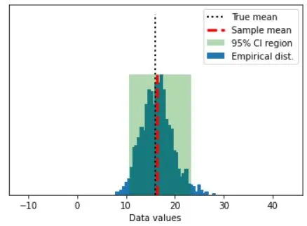
## graph everything
fig,ax = plt.subplots(1,1)

# start with histogram of resampled means
y,x = np.histogram(bootmeans,40)
y = y/max(y)
x = (x[:-1]+x[1:])/2
ax.bar(x,y)

y = np.array([ [confint[0],0],[confint[1],0],[confint[1],1],[confint[0],1] ])
p = Polygon(y,facecolor='g',alpha=.3)
ax.add_patch(p)

# now add the lines
ax.plot([popMean,popMean],[0, 1.5],'k:',linewidth=2)
ax.plot([samplemean,samplemean],[0, 1],'r--',linewidth=3)
ax.set_xlim([popMean-30, popMean+30])
ax.set_yticks([])
ax.set_xlabel('Data values')
ax.legend(('True mean','Sample mean','%g%% CI region'%confidence,'Empirical dist.'))
plt.show()

Confidence intervals - bootstrapping VS formula:

## compare against the analytic confidence interval

# compute confidence intervals
citmp = (1-confidence/100)/2
confint2 = samplemean + stats.t.ppf([citmp, 1-citmp],samplesize-1) * samplestd/np.sqrt(samplesize)

print('Empirical: %g - %g'%(confint[0],confint[1]))
print('Analytic:  %g - %g'%(confint2[0],confint2[1]))

OUT:
Empirical: 10.6507 - 23.3089
Analytic: 9.96088 - 22.5929

Real-World Example.

Finance is a field where uncertainty prevails, and making decisions based on incomplete information can lead to disastrous outcomes. Python Bootstrapping can be incredibly useful here. For instance, imagine an analyst who needs to determine the average daily return of a stock portfolio. A traditional approach would be to use a sample of the portfolio’s returns to calculate the confidence interval. However, classical methods have their limitations, such as having to assume normal distributions, which may not hold in finance.

Python Bootstrapping can address this problem of having small sample sizes and provides another way to estimate standard errors. It does not require any assumptions concerning the underlying distribution of the data, making it more reliable and accurate. Using Python Bootstrapping, the analyst can quickly determine the average daily return and evaluate the uncertainty surrounding it.

The steps to use Python Bootstrapping in finance are relatively simple. The first step is to obtain the data and then resample it with replacement to create the distribution. Next, calculate the average daily return, standard deviation, and t-statistics of the resampled distribution. Finally, use these statistics to calculate a confidence interval.

Interpreting the results of the Python Bootstrapping is almost the same as the classical approach. The confidence interval obtained from Python Bootstrapping tells us the range of values where the true population parameter is likely to lie. One of the significant advantages of Python Bootstrapping is that it provides the analyst with a range of values for the upper and lower bounds of the confidence interval.

Python Bootstrapping can be a valuable tool in finance as it provides a more accurate estimate of standard errors, gives better and more definite confidence intervals, and requires minimal assumptions concerning the underlying distribution. Furthermore, it can be used to conduct hypothesis tests and simulate distributions.

Conclusion.

Confidence intervals and bootstrapping are powerful tools for statistical inference. Python bootstrapping has been proven to be highly applicable in real-world scenarios. By using simulations, we can produce reliable confidence intervals even with complex data. By relying on these advanced techniques, we can bypass the limitations of classical methods. Ultimately, Python bootstrapping can help us make better decisions by providing more accurate, precise, and reliable estimates of population parameters. Therefore, it is essential to comprehend and use these statistical techniques to solve complex financial and other real-world problems.