Python Portfolio Allocation: Your Roadmap to Wealth Management Excellence!

In Finance, a Portfolio is a collection of Investments held by an investment company, financial institution or individual. Or you can define it as set of allocations in a variety of securities
Main Characteristics:
▪ Assets included in the Portfolio.
▪ Weights of the Portfolio Assets.

To make long story short, lets create our first trial portfolio using Python. We will use quandl to get market historical data, you can use any other source of information. We will chose popular tech stocks for our investment - Apple, Google, Amazon and IBM, set start and end dates for our investment and import the data.
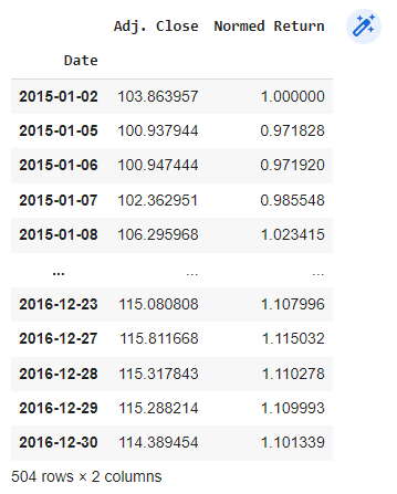
From 'Adjusted Close' daily column we will calculate 'Normed Return', which is cumulative daily returns for each stock - the total change in the investment price over a set time from the first day.

# pip install quandl
import pandas as pd
import quandl
import matplotlib.pyplot as plt
%matplotlib inline

start = pd.to_datetime('2015-01-01')
end = pd.to_datetime('2017-01-01')

aapl = quandl.get('WIKI/AAPL.11',start_date=start,end_date=end)
cisco = quandl.get('WIKI/CSCO.11',start_date=start,end_date=end)
ibm = quandl.get('WIKI/IBM.11',start_date=start,end_date=end)
amzn = quandl.get('WIKI/AMZN.11',start_date=start,end_date=end)

for stock_df in (aapl,cisco,ibm,amzn):
    stock_df['Normed Return'] = stock_df['Adj. Close']/stock_df.iloc[0]['Adj. Close']

aapl    

Allocations time is here and we implement the following allocations for our portfolio, percentages below should add up to 100% :
30% in Apple.
20% in Google(Alphabet).
30% in Amazon.
20% in IBM.

Then we calculate 'Allocations' column from 'Normed Return' column using percentages above. And now we are ready to invest our imaginary 1 million USD and check the results.

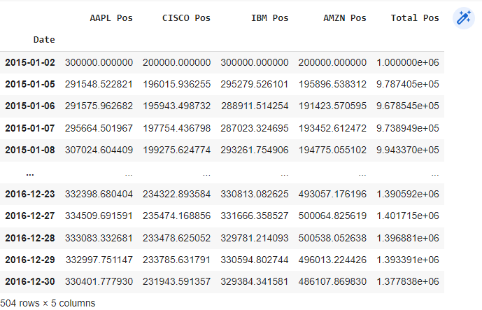
Results are calculated in 'portfolio_val' portfolio dataframe where we add 'Total Pos' column to display total portfolio value change.

#allocating
for stock_df,allo in zip([aapl,cisco,ibm,amzn],[.3,.2,.3,.2]):
    stock_df['Allocation'] = stock_df['Normed Return']*allo  

#investing
for stock_df in [aapl,cisco,ibm,amzn]:
    stock_df['Position Values'] = stock_df['Allocation']*1000000  

#creating portfolio dataframe    
portfolio_val = pd.concat([aapl['Position Values'],cisco['Position Values'],ibm['Position Values'],amzn['Position Values']],axis=1)
portfolio_val.columns = ['AAPL Pos','CISCO Pos','IBM Pos','AMZN Pos']
portfolio_val['Total Pos'] = portfolio_val.sum(axis=1)
portfolio_val

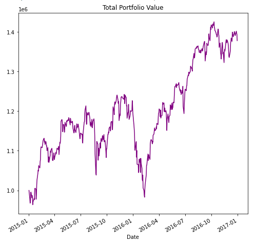
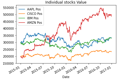
Now lets see dynamics of 'Total Portfolio Value' and individual stocks.

portfolio_val['Total Pos'].plot(figsize=(8,8), color='purple')
plt.title('Total Portfolio Value')

portfolio_val.drop('Total Pos',axis=1).plot(kind='line')
plt.title('Individual stocks Value')

Now we calculate main portfolio statistics which includes overall Cumulative Return, Average Daily Return and Daily Return standard deviation. Daily Return is just the percent returned from one day to the next.

# calculating Daily Return  
portfolio_val['Daily Return'] = portfolio_val['Total Pos'].pct_change(1)

# calculating Cumulative Return
cum_ret = 100 * (portfolio_val['Total Pos'][-1]/portfolio_val['Total Pos'][0] -1 )

# calculating Average Daily Return
day_ret_mean = portfolio_val['Daily Return'].mean()

# calculating Daily Return standard deviation
day_ret_std = portfolio_val['Daily Return'].std()


print(f'Our Cumulative return was {cum_ret} percent with Average Daily Return {day_ret_mean} and Daily return standard deviation {day_ret_std} ')

OUT: Our Cumulative return was 37.78375806982355 percent with Average Daily Return 0.0007086585746101822 and Daily return standard deviation 0.011947082021347087

The Sharpe Ratio is a method for calculating risk-adjusted return, and this ratio nowadays has become the industry standard for such calculations.
It was developed by Nobel laureate William F.Sharpe. The main idea is to implement the metric for most profitable and less volatile portfolio, the higher the ratio the better. General rule: Sharpe Ratio > 1 is usually considered as GOOD for investments, Ratio > 2 is VERY GOOD, Ratio > 3 is EXELLENT.
The formula is simple:
Sharpe ratio or SR = (Mean portfolio return − Risk-free rate) / (Standard deviation of portfolio return)

Annualized Sharpe Ratio or ASR = K-value * SR
where in our daily case of initial data K-value = sqrt(252) where 252 is equal to the number of trading or working days.
In case of weekly initial data K-value = sqrt(52), for monthly data K-value = sqrt(12).

IMPORTANT: Risk-free rate is rate you can get for your money without investments, e g on a usual bank savings account. In a example below we consider it equal to 0 to keep things simple, as most of the banks provide rates about zero today. You can easily adjust case below with non-zero Risk-free rate of your choice.

SR = portfolio_val['Daily Return'].mean()/portfolio_val['Daily Return'].std()
ASR = (252**0.5)*SR
print(f'For our portfolio SR = {SR} and ASR = {ASR} ')

OUT: For our portfolio SR = 0.05931645680040939 and ASR = 0.9416195600843358

Investment portfolio allocation with Python is a powerful approach that combines the principles of portfolio theory and the capabilities of Python programming. By utilizing it's extensive libraries and tools, investors can make informed decisions and optimize their investment portfolios.
Firstly, Python allows for efficient data analysis and manipulation, enabling investors to gather and analyze large amounts of financial data. This data-driven approach helps investors gain insights into asset performance, risk metrics, and correlations.
Secondly, Python provides various portfolio optimization techniques, such as mean-variance optimization, which helps investors find the optimal allocation of assets to maximize returns while minimizing risk.
Furthermore, Python's integration with financial APIs allows for real-time data updates, ensuring that investment decisions are based on the most current information.
It's visualization libraries, such as Matplotlib and Seaborn, enable investors to create insightful charts and graphs to visually analyze portfolio performance and asset allocation.
In addition, Python's flexibility and versatility make it suitable for implementing complex investment strategies, including factor investing, risk parity, and tactical asset allocation.
Overall, investment portfolio allocation with Python empowers investors to make data-driven, informed decisions, optimize their portfolios, and potentially enhance their investment returns while managing risk effectively.