How to optimize investment portfolio using Python.

The MPT or Modern Portfolio Theory is an investment theory made by Harry Markowitz based on the idea that risk-averse investors can construct portfolios to optimize or maximize expected return based on a given level of market risk, emphasizing that risk is an inherent part of higher reward. It is one of the most significant and influential economic theories dealing with financial investment.

Obtaining initial data.

Now lets import necessary Python libraries for our project. We will use quandl to get market historical data, you can use any other source of information. We will chose popular tech stocks for our investment - Apple, Google, Amazon and IBM, set interval dates for our investment and import the data.
We will create 'Adjusted Close' dataset, 'Daily returns' dataset and dataset with returns with allied log function - 'Log Returns'.

Using log returns instead of arithmetic returns will perform detrending/normalizing operation to the time series data. Log returns are convenient way to work with in many of the algorithms in financial area.

# pip install quandl
import numpy as np
import pandas as pd
import quandl
import matplotlib.pyplot as plt
%matplotlib inline

# setting the dates
start = pd.to_datetime('2016-01-01')
end = pd.to_datetime('2017-01-01')

# Getting tech stocks for our portfolio
aapl = quandl.get('WIKI/AAPL.11',start_date=start,end_date=end)
cisco = quandl.get('WIKI/CSCO.11',start_date=start,end_date=end)
ibm = quandl.get('WIKI/IBM.11',start_date=start,end_date=end)
amzn = quandl.get('WIKI/AMZN.11',start_date=start,end_date=end)

# creating stocks dataset
stocks = pd.concat([aapl,cisco,ibm,amzn],axis=1)
stocks.columns = ['aapl','cisco','ibm','amzn']


# creating stocks daily return dataset
stock_daily_ret = stocks.pct_change(1)
stock_daily_ret.head()

# applying log function to returns
log_ret = np.log(stocks/stocks.shift(1))

log_ret  

Log returns dataset:

Portfolio optimization using Monte Carlo Simulation.

The script below will generate certain amount of attempts setting random weights to stocks in our investment portfolio. In our case we consider 10000 attempts as optimal amount, you can adjust it according to your case needs. For all the attempts Sharpe Ratio is calculated together with Expected Return and Expected Variance. Then we just select the case with maximum Sharpe Ratio and corresponding portfolio optimal assets weights.

num_ports = 10000

all_weights = np.zeros((num_ports,len(stocks.columns)))
ret_arr = np.zeros(num_ports)
vol_arr = np.zeros(num_ports)
sharpe_arr = np.zeros(num_ports)

for ind in range(num_ports):

    # Create Random Weights
    weights = np.array(np.random.random(4))

    # Rebalance Weights
    weights = weights / np.sum(weights)
   
    # Save Weights
    all_weights[ind,:] = weights

    # Expected Return
    ret_arr[ind] = np.sum((log_ret.mean() * weights) *252)

    # Expected Variance
    vol_arr[ind] = np.sqrt(np.dot(weights.T, np.dot(log_ret.cov() * 252, weights)))

    # Sharpe Ratio
    sharpe_arr[ind] = ret_arr[ind]/vol_arr[ind]

sharpemax = sharpe_arr.max()  
sharpemaxposition = sharpe_arr.argmax()
optimalweights = all_weights[sharpemaxposition,:]
max_sr_ret = ret_arr[sharpemaxposition]
max_sr_vol = vol_arr[sharpemaxposition]


print(f'Maximum Sharpe Ratio found {sharpemax} at position {sharpemaxposition} ')
print(f'And optimal weights for portfolio {optimalweights} ')

OUT:
Maximum Sharpe Ratio found 1.243574241330179 at position 448
And optimal weights for portfolio [0.03471546 0.13234325 0.73066413 0.10227716]

Plotting the data.

Now lets plot the Bullet chart with all the simulated data and define optimal portfolio solution with maximum Sharpe Ratio as a red dot.

plt.figure(figsize=(12,8))
plt.scatter(vol_arr,ret_arr,c=sharpe_arr,cmap='viridis')
plt.colorbar(label='Sharpe Ratio')
plt.xlabel('Volatility')
plt.ylabel('Return')

# Add red dot for max SR
plt.scatter(max_sr_vol,max_sr_ret,c='red',s=50,edgecolors='black')

Portfolio Mathematical Optimization.

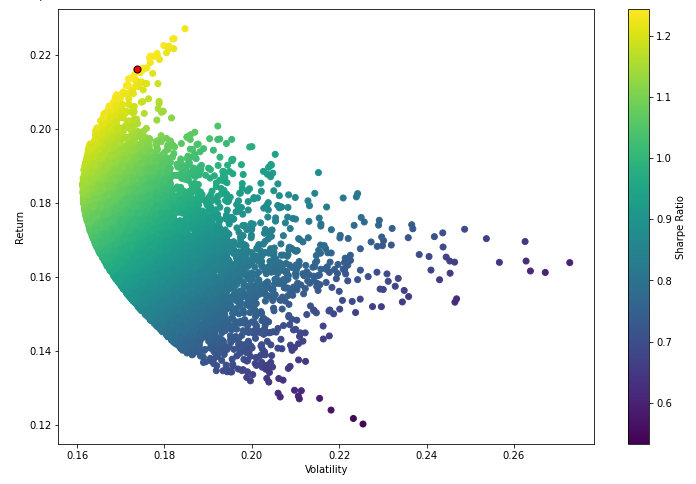
Generating random weights method provides quite good results for our optimization task, but depending on portfolio size it can take huge amount of time and a lot of fine tuning iterations to set optimal number of attemts.

The next method we suggest is much faster and more optimal, it uses Mathematical Optimization or simply minimize function from Python scipy library. At the end we will get the solution with optimal Sharpe Ratio and corresponding portfolio assets weights as in the previous Monte Carlo Simulation case. It is interesting to compare results between both cases.

from scipy.optimize import minimize

def get_ret_vol_sr(weights):
    """
    Takes in weights, returns array or return,volatility, sharpe ratio
    """
    weights = np.array(weights)
    ret = np.sum(log_ret.mean() * weights) * 252
    vol = np.sqrt(np.dot(weights.T, np.dot(log_ret.cov() * 252, weights)))
    sr = ret/vol
    return np.array([ret,vol,sr])

def neg_sharpe(weights):
    return  get_ret_vol_sr(weights)[2] * -1

# Contraints
def check_sum(weights):
    '''
    Returns 0 if sum of weights is 1.0
    '''
    return np.sum(weights) - 1

# By convention of minimize function it should be a function that returns zero for conditions
cons = ({'type':'eq','fun': check_sum})

# 0-1 bounds for each weight
bounds = ((0, 1), (0, 1), (0, 1), (0, 1))

# Initial Guess (equal distribution)
init_guess = [0.25,0.25,0.25,0.25]

# Sequential Least SQuares Programming (SLSQP).
opt_results = minimize(neg_sharpe,init_guess,method='SLSQP',bounds=bounds,constraints=cons)

optimalweights = opt_results.x

optimalresults = get_ret_vol_sr(opt_results.x)

print(f'Optimal portfolio weights are {optimalweights} ')
print(f'Maximum Sharpe Ratio found {optimalresults[2]} ')

OUT:
Optimal portfolio weights are [0.0085194 0.11503318 0.75099555 0.12545186] Maximum Sharpe Ratio found 1.2448937848938475

Defining the Efficient Frontier.

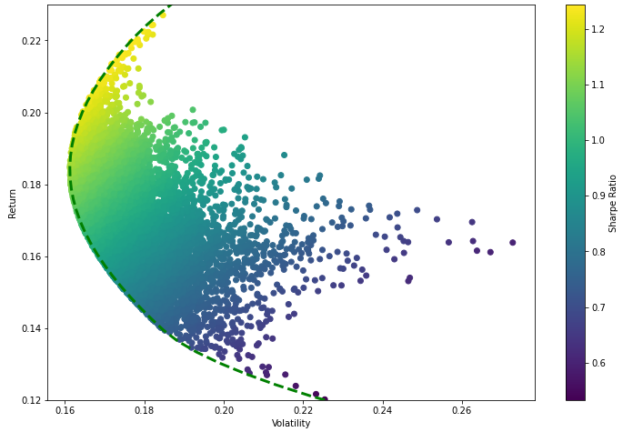
The set of optimal portfolios that provides the highest expected return for a determined level of risk or the lowest risk for a given level of expected return is called the efficient frontier. Portfolios on the bullet chart that lie below the efficient frontier are sub-optimal, because they do not provide enough return for the level of risk. Portfolios that cluster to the right of the efficient frontier are also sub-optimal, because they have a higher level of risk for the defined rate of return.

# Creating a linspace number of points to calculate x on a specified range
frontier_y = np.linspace(0,0.3,100) # Adjust 100 to a lower number for slower computers!


def minimize_volatility(weights):
    return  get_ret_vol_sr(weights)[1]


frontier_volatility = []

for possible_return in frontier_y:
    # function for return
    cons = ({'type':'eq','fun': check_sum},
            {'type':'eq','fun': lambda w: get_ret_vol_sr(w)[0] - possible_return})
   
    result = minimize(minimize_volatility,init_guess,method='SLSQP',bounds=bounds,constraints=cons)
   
    frontier_volatility.append(result['fun'])

plt.figure(figsize=(12,8))
plt.scatter(vol_arr,ret_arr,c=sharpe_arr,cmap='viridis')
plt.colorbar(label='Sharpe Ratio')
plt.xlabel('Volatility')
plt.ylabel('Return')
plt.ylim((0.12,0.23))


# Add frontier line
plt.plot(frontier_volatility,frontier_y,'g--',linewidth=3)