CAPM Redefined: Harnessing Python for Precision and Performance!.

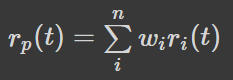
As a portfolio is a set of weighted securities, return of our portfolio is described by the returns of it's securities with their corresponding weights by formula:

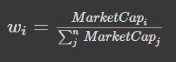
We can imagine the entire market as a portfolio, e g S&P500, and the weight of company i can be described as its capitalization (number of shares multiplied by shere price) divided by market capitalization as stated in formula:

The CAPM equation for a portfolio describes the return of certain individual stock i:

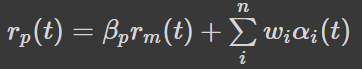
As seen from equation above Capital Asset Pricing Model can be described as simple linear regression with alpha and beta coefficients. The return of the stock is equivalent to the return of the market multiplied by beta factor plus some residual alpha term at time t. If beta=1 then stock i moves in line with the market. The CAPM expects alpha to be zero, or close to zero in real life. And that alpha is random and cannot be predicted.

Ecpecting alpha to be zero means that you cannot beat the market !!! But if we can predict the alpha with certain confidence, e g more than 50%, this means we can invest more efficient than just investing in the total market.

Now lets import necessary Python libraries for our project. We will use pandas_datareader to get market historical data, you can use any other source of information. We will chose Apple stocks data and check its behaviour against market, which is S&P500 in this case (SPY ETF). At the end we will calculate alpha and beta coefficients for Capital Asset Pricing Model.

from scipy import stats
import pandas as pd
import pandas_datareader as web
import matplotlib.pyplot as plt
%matplotlib inline


start = pd.to_datetime('2020-01-01')
end = pd.to_datetime('2022-01-01')

spy_etf = web.DataReader('SPY','stooq', start, end)
aapl = web.DataReader('AAPL','stooq',start,end)


spy_etf.sort_index(inplace=True)
aapl.sort_index(inplace=True)

aapl['Cumulative'] = aapl['Close']/aapl['Close'].iloc[0]
spy_etf['Cumulative'] = spy_etf['Close']/spy_etf['Close'].iloc[0]
aapl['Cumulative'].plot(label='AAPL',figsize=(10,8))
spy_etf['Cumulative'].plot(label='SPY Index')
plt.legend()
plt.title('Cumulative Return') 

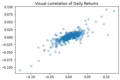
Now lets calculate 'Daily Return' column for our dataframes and see correlation betwenn data for different APPL and S&P500.

aapl['Daily Return'] = aapl['Close'].pct_change(1)
spy_etf['Daily Return'] = spy_etf['Close'].pct_change(1)
plt.scatter(aapl['Daily Return'],spy_etf['Daily Return'],alpha=0.3)
plt.title('Visual correlation of Daily Returns')

Then using linear regression from SCIPY library we can calculate alpha and beta along with r_value.

beta,alpha,r_value,p_value,std_err = stats.linregress(aapl['Daily Return'].iloc[1:],spy_etf['Daily Return'].iloc[1:])

print(f"Beta coefficient is equal to {beta}, alpha is equal to {alpha}, r_value is equal to {r_value}")

OUT: Beta coefficient is equal to 0.5398027692578261, alpha is equal to -0.00014317322452608264, r_value is equal to 0.7976803835511338